

Ⅰ. Introduction
The temporal variability of water quality parameters is information critical for efficient watershed management (Montgomery et al., 2007; Horsburgh et al., 2009). NPS pollutants are loaded to waterbodies with rainfall events that may last several days. In addition, the transport of NPS pollutants is complicated with hydrological processes that greatly vary over time, even in an event. Thus, a frequent monitoring is often required when assessing NPS pollution and developing water quality management plans (Scholefield et al., 2005; Houser et al., 2006; Jordan et al., 2007). However, frequent NPS monitoring is often prohibitive in terms of time and effort.
The use of high-frequency water quality sensors can be one of the solutions for the cost issue of NPS monitoring, but many of water quality parameters such as suspended solids (SS) and total phosphorus (T-P) still require extensive equipment and lab tests to be quantified (Jones et al., 2011, Villa et al., 2019). In this context, surrogate monitoring can be an efficient alternative. Previous studies have tried to predict the water quality parameters with accessible parameters such as pH, dissolved oxygen (DO), temperature using traditional statistical techniques such as multiple linear regression (MLR) (Çamdevýren et al., 2005; Chenini and Khemiri, 2009; DeForest et al., 2018). Some of them showed that SS and T-P is closely associated with turbidity and discharge rates of a river (Jones et al., 2011; Ziegler et al., 2011). It is a relative measure of light diffraction in water caused by particulate form, and the use of turbidity as a surrogate parameter to estimate T-P is based on that T-P transported in streams predominantly particulate form (Settle et al., 2007; Ruegner et al., 2013). Moreover, Johanna et al. (2014) predicted SS, particulate organic carbon, and particulate nitrogen from turbidity, flow discharge rate, and rainfall depth using MLR. Although, MLR is a simple statistical method to use (Jones et al., 2011; Ziegler et al., 2011; Johanna et al., 2014), and its application is limited to linear relationships, and it is known to be very sensitive to outliers (Chatterjee and Hadi, 1988).
The use of machine learning techniques such as random forest (RF) became affordable with recent advances made in computing resources and techniques, and they have been employed as an analysis tool for hydrologic research (Rodriguez-Galiano et al., 2014; Singh et al., 2017). The RF is a computational algorithm that can predict the values of continuous variables from continuous and/or categorical predictor variables by constructing a decision tree or classifying data (Razi et al., 2005). The algorithm is known not to overfit and efficient in predicting irregular variables that exhibit little periodicity (Diaz-Uriate and de Andres, 2006).
This study explored the potential of the RF algorithm as a tool to efficiently identify primary variables that can serve as surrogate for NPS pollutants. We developed prediction models using MLR (traditional statistical model) and RF (the latest statistical data mining technique) and compared their performance to demonstrate their capacities and potentials. This study focused on SS and T-P that are common NPS pollutants in Korea.
Ⅱ. Material and methods
1. Study areas and NPS monitoring
This study has monitored SS and T-P at the outlet of a catchment, Wol-jeong (WJ), located within the Pungyeongjeongcheon watershed in Korea for two years, from 01/01/2017 and 12/31/2018 (Fig. 1). WJ is mostly covered by agricultural land uses (86%) including rice paddy fields and upland. The mean annual temperature and precipitation of the study catchment are 13.8°C and 1,391 mm, respectively.
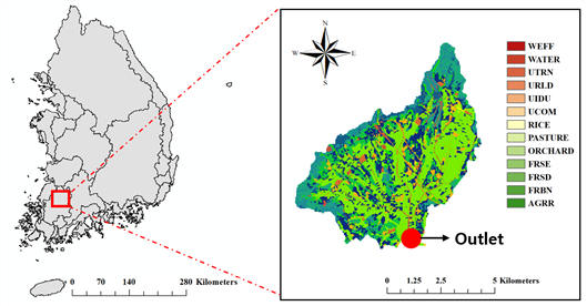
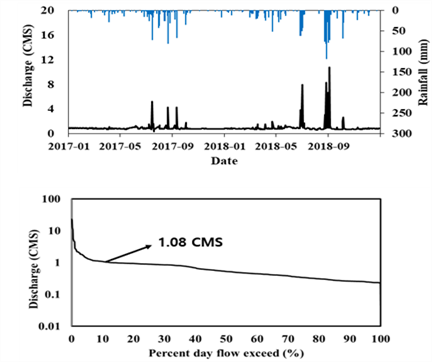
A set of water pressure sensor and logger (OTT Orpheus mini, Germany) was installed to monitor the level of streamflow, and the velocity (VALEPORT model 002, UK) and cross section of flow were measured six times during the monitoring period. The flow level measurements were converted to discharge data using a flow rating curve developed for the outlet of the study catchment. A digital turbidity sensor (FTS DTS-12, Canada) was installed to monitor the turbidity of flow at the monitoring site (or the outlet). The flow duration curve was then developed from flow observations and the flow conditions was seperated using Table 1. Then, we separated the flow conditions into high-flow periods (the exceedance probability equal to or less than 10%) and low-flow ones (the exceedance probability greater than 10%) so that the flow-dependent behavior of NPS pollutant transport can be examined in the study. Stormwater samples were taken every hour in the first 24 hours of a storm event using an automatic sampler (ISCO portable sampler 6712, USA), and the sampling interval was increased to 6 hours for the rest of the event. The concentrations of SS and T-P were analyzed in a laboratory according to the standard water pollution test method (APHA, 2001). The monitored water quality variables and predictors such as turbidity and runoff discharge rates are summarized in Table 2.
2. Surrogate model development
The potential relationships between the pollutants of interest (SS and T-P) and the primary environmental variables (discharge rates and turbidity) were explored using the MLR and RF methods. RF is the combination of tree-based classification methods such as a regression tree developed by Breiman, (2001). The processes of growing regression trees can be summarized into two steps. First, data of interest are split into multiple tree branches in the way toward minimizing least-square deviations between observed and predicted variables, which is called the optimal split (OPs) (Hasanipanah et al., 2017). The split is calculated as the difference of variance between the mother node and the left child node, and the right child node is maximized by using Eqs. 1 and 2 (Ließ et al., 2012; Granata et al., 2017).
where R(t) is the variance in a node t, which is divided into the left and right child nodes, tl and tr. n is the number of observations, and  is the mean value of the predicted variable.
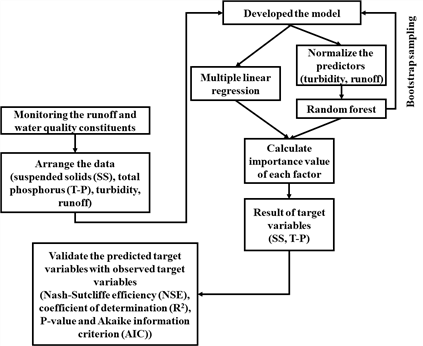
Once tree branches are constructed in the first step, RF prunes the trees by removing nodes that have low explanatory power. Here, the existence of nodes that may be removed imply overfitting. An overfitted model does not sensitively respond to newly added data, and it creates additional uncertainty to the prediction (Breiman et al., 1984). Thus, the pruning process is necessary to reduce prediction uncertainty. The overall procedures of predicting SS and T-P using the MLR and RF models are presented in Fig. 2.
The RF uses a bagging technique with a randomized subset of variables, which is mathematically described using Eq. 3 (Prasad et al., 2006).
where  is a RF prediction, K is the number of trees (or branches), and T(x) is the result of each regression tree.
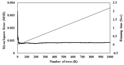
The node size (five) was adapted from literature (Wang et al., 2015) and the’mtry’ is the number of predictors to select at random for each split in the tree model. However, we used only two variables in this study, so we used’mtry’ of two. The RF model calculates the relative importance of each parameter using the Gini impurity (GI) and mean square error (MSE) statistics. GI quantifies the quality of each split, and MSE calculates the mean decrease of prediction accuracy (Breiman, 2001; Ouedraogo et al., 2018). The GI method is used to calculate the quality of each split for the variables in a tree model and calculate the mean decrease using MSE due to splits on every predictor (Breiman, 2001). In this study, we found that K of 100 is enough to stabilize the MSE. However, the running time of RF slightly increased until K value hit 1,000. We selected K value of 1,000 while still providing reasonably short computing time (Fig. 3). The relative importance was calculated by running the RF algorithm 100 times and then averaging the importance rates calculated from the iterations.
It is known that one of the considerations in the machine learning technique is that training variables with different range affects the learning rates and it can be crucial problems with prediction performance (Ioffe and Szegedy, 2015). For example, turbidity ranges from 6.6 to 383 NTU, and runoff ranges from 0.6 to 3.2 m3/s in this study. Then, the turbidity and runoff discharge rate data were normalized into the range from 0 to 1 using Eq. 4 to assure that each variable can have the similar level of explanatory power in the analysis.
where  is the normalized value of the data set (range of 0 to 1) and
  is the original value.
The flow observations made from 2017 to 2018 showed that the flow discharge rate of 1.08 m3/s correspond to the 10% discharge of the study catchment (Fig. 4). The threshold rate of 1.08 m3/s was used to separate discharge into high and low flow, and then the models were separately applied to the two flow regimes.
The performance of the MLR and RF models was evaluated with the split-sample scheme of 80/20 (80% for training and 20% for validation; Afendras and Markatou, 2019). To validate the models, we used four different statistics and criteria: the Nash-Sutcliffe efficiency (NSE) coefficient, the coefficients of determination (R2), p-value (P), and the Akaike information criterion (AIC) (Nash and Sutcliffe, 1970; Akaike, 1973; Snipes and Taylor, 2014).
where Xi and Yi is the predicted value and observed values from site i and n is the number of samples. In the AIC method, k represents the number of parameters, and L is the likelihood function, which represent the model fit and it should represented by log-value to limit the maximum value of model fit.
A lower AIC score is interpreted as a more accurate model. The p-value is defined as the probability (Pr), under the null htpothesis H about the unknown distribution of the T. If the p-value shows very small value, then the statistical significance is thought to be very large. On the other hand, the criteria commonly set to 0.05, 0.01, 0.005, or 0.001 and we choose 0.001 as criteria in this study.
Ⅲ. Results and discussion
The comparison between observation and prediction result was conducted with normalized value, and the normalized SS and T-P prediction results of the MLR and RF models are compared with the normalized observation values in Fig. 5 and Table 3. Overall, the MLR model prediction of SS and T-P in the low and high flow conditions were acceptable with R2 and NSE greater than 0.5, except T-P in low flow condition. The T-P prediction for the low flow condition shows acceptable R2 but low NSE. The reason for this result is that T-P in agricultural area shows high concentrations for high flow conditions during farming period (Villa et al., 2019). Thus, high flow conditions shows acceptable prediction performance with high concentrations of T-P which shows high fluctuations and low flow condition shows unacceptable prediction performance due to low concentrations of T-P. In general, SS and T-P were more accurately predicted by the MLR models when runoff discharge is relatively large (or the high flow condition). The RF model provided accuracy and its patterns similar to that of the MLR model.
Table 3
Performance evaluation of the MLR and RF models in predicting SS and T-P concentrations
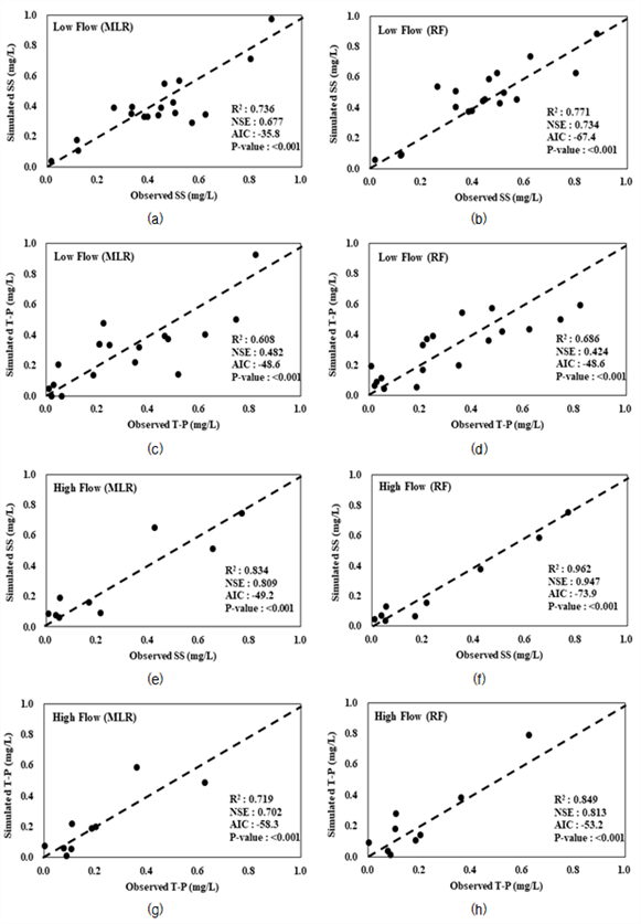
Fig. 5
Comparison between the NPS pollutants observed and simulated using the MLR and RF models (a) SS using MLR in low flow condition; (b) SS using RF in low flow condition; (c) T-P using MLR in low flow condition; (d) T-P using RF in low flow condition. (e) SS using MLR in high flow condition; (f) SS using RF in high flow condition; (g) T-P using MLR in high flow condition; (h) T-P using RF in high flow condition
As both models provided similar accuracy when predicting SS and T-P from turbidity and runoff discharge rates, their performance was further investigated in terms of AIC values (Table 3). The AIC values of the RF model are lower than those of the MLR model, indicating that the RF model is more suitable for predicting SS and T-P that the MLR model in this study.
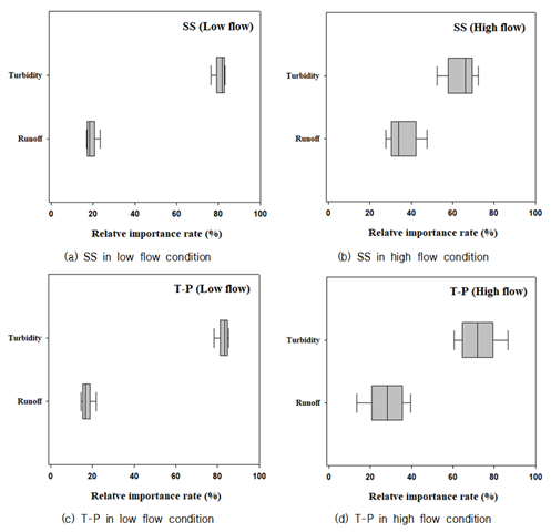
The relative importance of the primary environmental variables, runoff discharge rates and turbidity, to predict SS and T-P was quantified as part of the RF modeling (Fig. 6). The analysis of relative importance showed that turbidity was more closely associated with the SS and T-P concentrations than discharge rates with importance rates ranging from 52% to 86% depending on the flow conditions. As mentioned above, the runoff in high flow condition shows higher relative importance than low flow condition, which is related to the high concentrations of T-P in farming period.
Ⅳ. Conclusions
This study explored the potential of the MLR and RF model as a tool to identify surrogate environmental variables in two different flow conditions for the concentrations of NPS pollutants such as SS and T-P in agricultural sub-watershed. The performance of the MLR and RF models was evaluated with the 80% for training set and 20% for validation set. Both MLR and RF models provided acceptable performance when predicting SS and T-P in the high-flow condition. The relative importance rate analysis showed that turbidity had relatively high explanatory power (52% to 86%) than runoff discharge rates. Moreover, the runoff in high flow condition shows higher relative importance than low flow condition, which is related to the high concentrations of T-P in farming period. This study demonstrated the machine learning techniques could help to improve the efficiency of NPS pollutant monitoring and prediction by identifying fundamental environmental variables that are relatively easily obtained but still closely related to the NPS pollutants. The results also showed that turbidity could serve as a surrogate water quality parameter for SS and T-P concentrations at acceptable accuracy levels.