

Ⅰ. INTRODUCTION
Evapotranspiration is one of the hydrologic cycle components and combines two distinct processes which are the evaporation of water directly from the ground surface and transpiration through the plants’ stomata (Allen et al., 2006). Knowledge of the reference crop evapotranspiration (ETo) is very important in various fields of water resources such as estimation of crop water requirements, scheduling of irrigation water application, modeling of rainfall-runoff process and evaluation of land suitability (Djaman, et al., 2018). Because of its significance, various indirect and direct methods have been used to determine ETo.
Direct methods include field measurements using lysimeters and pan evaporimeters to quantify evapotranspiration (Parisi et al., 2009; Lu et al., 2018), however, these methods are time-consuming. Furthermore, time, labor and high skill for data collection and communication are required to improve estimates and spatial interpolation, which may be inappropriate for large-scale studies (Palayasoot, 1965). On the other hand, methods using micro-meteorological measurements such as the energy balance Bowen ratio and eddy covariance flux measurement systems have also been employed to measure surface heat fluxes but these are expensive and complex, both of which limit their wide applicability (Drexler et al., 2004).
Due to limitations associated with direct methods, the adoption of indirect methods of physical mathematical formulations has become a preferred and practical alternative to ETo estimation (Allen et al., 2011). ETo is a complex process which is dependent on several interacting climatological factors, such as temperature, humidity, wind speed and radiation. The lack of physical understanding of the ETo process and the unavailability of all relevant data results in inaccurate estimation of ETo (Vyas and Subbaiah, 2016). Consequently, significant research activities have been carried out to develop and/or implement reliable and accurate prediction models that use observed weather data (air temperature, relative humidity, solar radiation and wind speed) as inputs to estimate ETo (Jensen et al., 1990; Allen et al., 1998; Jennifer and Sudheer, 2001; George et al., 2002; Itenfisu et al., 2003).
The Penman-Monteith equation (FAO 56-PM) is maintained as the single standard method recommended by the FAO for the computation of ETo from complete meteorological data (Smith et al., 1992; Allen et al., 2006). Several models such as Hargreaves & Blaney-Criddle and other models have been proposed to predict ETo, but Traoré et al. (2008) reported that these models do not have universal consensus for different climatic conditions. Even though its modeling accuracy is well known, the main shortcoming of the FAO 56-PM method is its requirement of a large number of meteorological data that are not always available in many locations. For this reason, numerous attempts have been tried to overcome difficulties associated with data availability for ET estimation (Dai et al., 2009).
To address this, past studies investigated the application of Artificial Neural Networks (ANNs) and assessed their performance with limited number of datasets rather than a full set of data (minimum, average & maximum air temperature, relative humidity, wind speed and solar radiation). ANNs have been intensively used in modeling complex nonlinear processes (e.g., rainfall-runoff, stream flow, ground water, precipitation and evapotranspiration) because they have the ability to map the input-output relationships without a complete understanding of the physical processes (Choi et al., 2018). Lee et al. (2010) showed the good performance of ANNs in estimating future reference crop evapotranspiration. Abedi-Koupai et al. (2009) evaluated the performance of ANNs with the conventional methods (Penman, Penman-Monteith, Stanghellini and Fynn) to estimate reference evapotranspiration and they found that the efficiency value of ANNs was superior than others. Sudheer and Jain (2003) and Zanetti et al. (2007) in their ET estimation simplified the neural network inputs to air temperature, extraterrestrial solar radiation and daily light hours. Khoob (2008) used similar input sets but without the daily light data for successfully estimating ET in Iran.
The objectives of this study were to adopt a Backpropagation neural network (BPNN) model to calculate daily ETo from different input combinations (minimum, average & maximum air temperature, relative humidity, wind speed and solar radiation) and to assess the computational performance of ETo values between BPNN and Multiple Linear Regression (MLR).
Ⅱ. MATERIALS AND METHODS
1. Description of Study area and Meteorological data
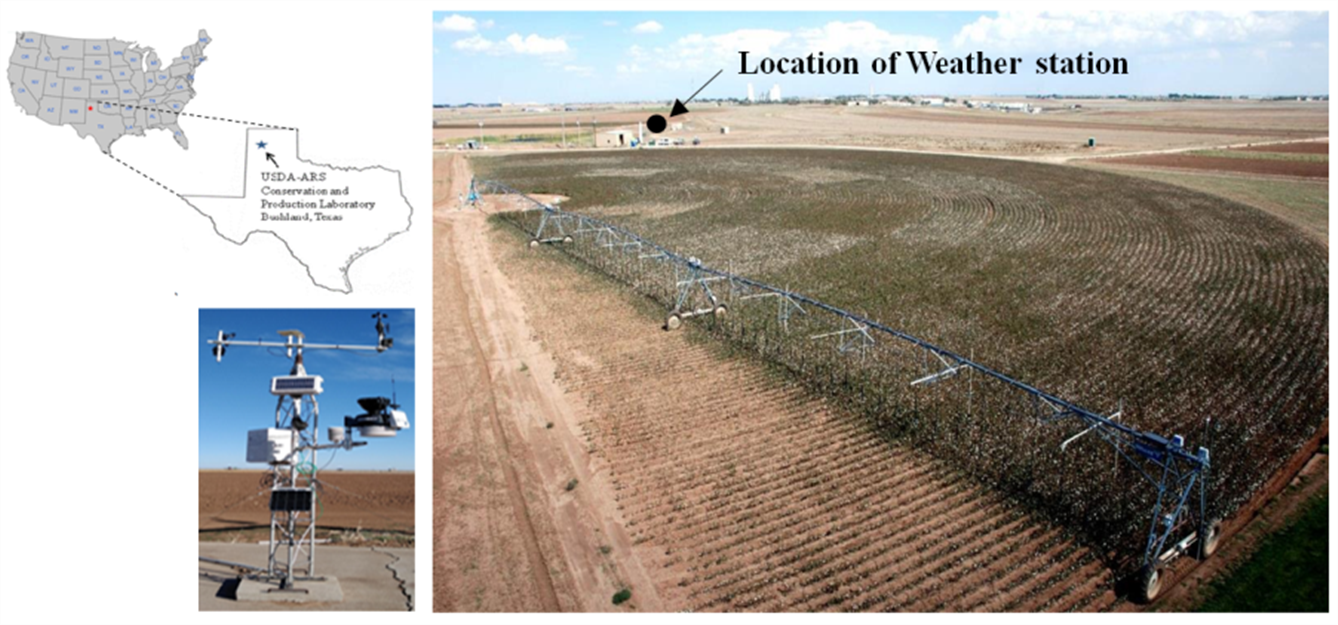
A total of six meteorological variables were collected from a weather station which was located at the experimental station in USDA Agricultural Research Service Conservation and Production Research Laboratory, Bushland, Texas, USA (35° 11’ N, 102° 6’ W, 1,170 m above MSL) (Fig. 1). Data from periods (May – December, 2010, January – December, 2012 and January, 2014 – October, 2017) were used and any faulty data due to sensor malfunction were deleted. All required data, average, minimum and maximum air temperature (Tavg, Tmin and Tmax, °C), relative humidity (RH, %), wind speed (WS, m/s) and solar radiation (SR, watt/m2), were measured at 6 second intervals, reported as 15 minutes mean values from a weather station, and then stored in a Datalogger (Campbell Scientific, CR3000, Logan, Utah, USA). Sensors used were temperature & relative humidity sensor (HC2S3, Rotronic, Hauppauge, New York, USA), pyranometer (LI200-RX, LI-COR, Lincoln, Nebraska, USA), and wind sentry set (Model 03002-L, R.M. Young, Traverse City, Michigan, USA).
2. Computation of reference crop evapotranspiration using the FAO 56-PM equation
The FAO 56-PM equation was developed to quantify the amount of water loss from soil surface and plant leaf through evaporation and transpiration. This equation accounts for aerodynamic as well as physiological parameters and requires large data inputs (Tmin, Tavg, Tmax, WS, RH and SR). The equation is as follows (Allen et al., 1998):
where ETo is reference crop evapotranspiration [mm day-1], Rn is net radiation at the crop surface [MJ m-2 day-1], G is soil heat flux density [MJ m-2 day-1], T is average daily air temperature at 2 m height [°C], u2 is wind speed at 2 m height [m s-1], es is saturation vapor pressure [kPa], ea is actual vapor pressure [kPa], (es-ea) is saturation vapor pressure deficit [kPa], Δ is slope vapor pressure curve [kPa °C-1], and γ is Psychrometric constant [kPa °C-1].
The FAO 56-PM equation requires daily data as inputs, therefore, all necessary data collected form a weather station were converted from every 15 minutes to daily averages (Tmin, Tavg, Tmax, RH and WS) and sums (SR) to apply to the FAO 56-PM equation.
3. Application of BPNN and MLR models
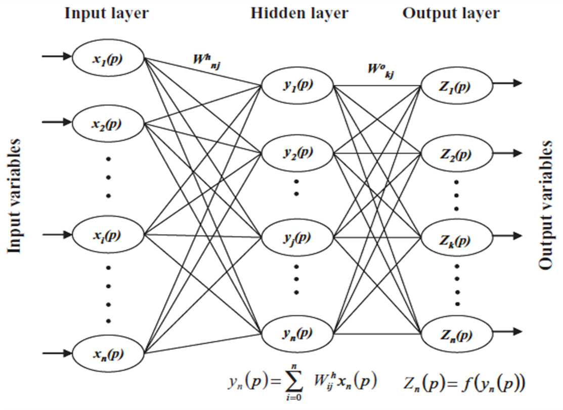
The Multi-Layer Perceptron (MLP), a traditional Artificial Neural Network, is known as the common, effective and successful neural network architecture which uses a supervised learning and technique called Backpropagation (BP) algorithm. Backpropagation neural network (BPNN) is by far the most popular (Haykin, 1998), performs parallel training for improving the efficiency of MLP networks, and derives the network error which is fed back into the network model and used to adjust the weights (Kecman, 2001; Mia et al., 2015). The MLP consists of at least three layers, an input layer, one or more hidden layer, and an output layer. Adjustable weights are used to connect the nodes between adjacent layers and optimized by the training algorithm to obtain the desired results. Through that process, the error in prediction decreases with each iteration, succeeds when the neural network model reaches the specified level of accuracy and produces the desired outputs (Kim et al., 2008). First of all, this study begun with three layer learning network which consists of an input layer, a hidden layer and an output layer (Fig. 2), but during the training procedure, more than one hidden layers were evaluated to calculate the weighted inputs with activation functions to produce the better outputs. In designing a robust and accurate ANN model, the modeler must address a number of important factors, including the type and structure of the neural network, the input prediction variables used, and data pre-processing. This was generally accomplished through a combination of best professional judgment, heuristic rules, and trial & error (Laaboudi et al., 2012). The governing factors in BPNN includes: a number of hidden layers, a number of hidden processing elements (PEs), the transfer function (e.g., sigmoid, tan-sigmoid), learning algorithm (e.g., Delta, extended DBD) and learning parameters (e.g., learning rate, momentum factor, initial weights) (Basheer and Hajmeer, 2000; Maier and Dandy, 2000). Depending on the problem being solved, the success of training varies with selected factors.
Among all six variables, its correlative regression with ETo was determined. Different combinations of input variables (number of combinations) were used in this study, 1, 2, 3, 4, 5 and 6 variables. The datasets of the following variables Tmin, Tavg, Tmax, RH, WS and RS, were used as the inputs and ETo was used as the output. They were all daily averaged. Except for one individual variable used as an input, the rest of input combinations (two, three, four, five and six variables) were prepared to match solar radiation, which has the highest correlation regression with ETo, with the others, which has the relatively high correlations (Table 1). A total of 20 combinations (from C1 to C20) were prepared to determine their best network configuration and regression equation for BPNN and MLR. In further explanation, a combination 1 (C1) to a combination 6 (C6) has only one variable defined as input and a combination 7 (C7) to a combination 11 (C11) has two variables as inputs as per high correlation with ETo.
Table 1
Different combinations of input variables and its correspondent output variable
To consider ANN modeling valid without manipulating data and/or evidence of contradictory results, all data used in this study was divided into three sets, one for the training, the other for the validation of the trained results, and another for the testing of the trained-validated results. A total of 1,633 datasets from 2010, 2012, 2014 to 2017 years were used, and 62% of data for network training, 8% for validation and 30% for testing were assigned, respectively. All meteorological input and output variables were standardized in the range of 0 to 1 using the Min-Max normalization method (Choi et al., 2018) and then partitioned using K-fold cross validation.
There is no established methodology for the selection of modeling parameters, such as the appropriate network architecture (the number of input, hidden and output layers), Processing Elements (PEs) in the hidden layer, the momentum, the learning rate, the learning rule and the transfer function in BPNN (Choi et al., 2018). Therefore, model convergence was based on the error function and exhibited any deviation between the predictions taken from corresponding target output values as the sum of the squares of the deviations. Training proceeded until the error was reduced to a desired minimum threshold. The most commonly used stopping criterion for neural network training was the sum-of-squared-error (SSE) which is presented in Equation (2) (Choi et al., 2018).
where n is the number of output,  is the measured output and
  is the predicted output.
A PC-based neural network application software, NeuralWorks Professional II/Plus (Neuralworks®, Carnegie, Pennsylvania, USA) used in this study, allows users to adjust key network and training parameters in BPNN. Modifications are preferred to determine the best combination for solving the particular problem. Given the number of possible parameter combinations, the possibility of finding the correct combination of parameter settings, given a random starting point, is unlikely and is based primarily on chance (Kim et al., 2008).
MLR techniques can be used to model ETo in terms of the local climatological parameters. The general purpose of the MLR model is to learn more about the relationship between several independent or predictor variables and a dependent or criterion variable. In MLR analysis, the values of ETo were used as the dependent variable, while each combinations was used as independent variables to derive the coefficients in the MLR model. The regression equations were generated with the aid of Microsoft Excel in this study.
4. Performance evaluation criteria
The performance of BPNN and MLR models was evaluated by comparing their predictive accuracies with the ETo values using Microsoft excel. The performance was characterized based on the following statistical criteria, which are R2 (coefficient of determination), RMSE (root mean square error) and NSE (Nash-Sutcliffe efficiency) (Equation 3-5).
where,  and
and  represent the FAO 56-PM estimate and its average for ith value;
  and
and  represent the BPNN (MLR) computed values and their average for ith value; N represents the number of data considered.
Ⅲ. RESULTS AND DISCUSSION
1. Meteorological condition of study area
The study area (Bushland, Texas, USA) has the meteorological condition which is categorized as semi-arid and has extremely variable precipitation temporally and spatially, which ranges from 400 to 560 mm. The area also has high evaporative demand, which is approximately 2,500 mm per year based on the Class A pan evaporation. This can be explained by high solar radiation, high vapor pressure deficit and strong regional advection. The monthly meteorological conditions in Bushland are plotted in Fig. 3.
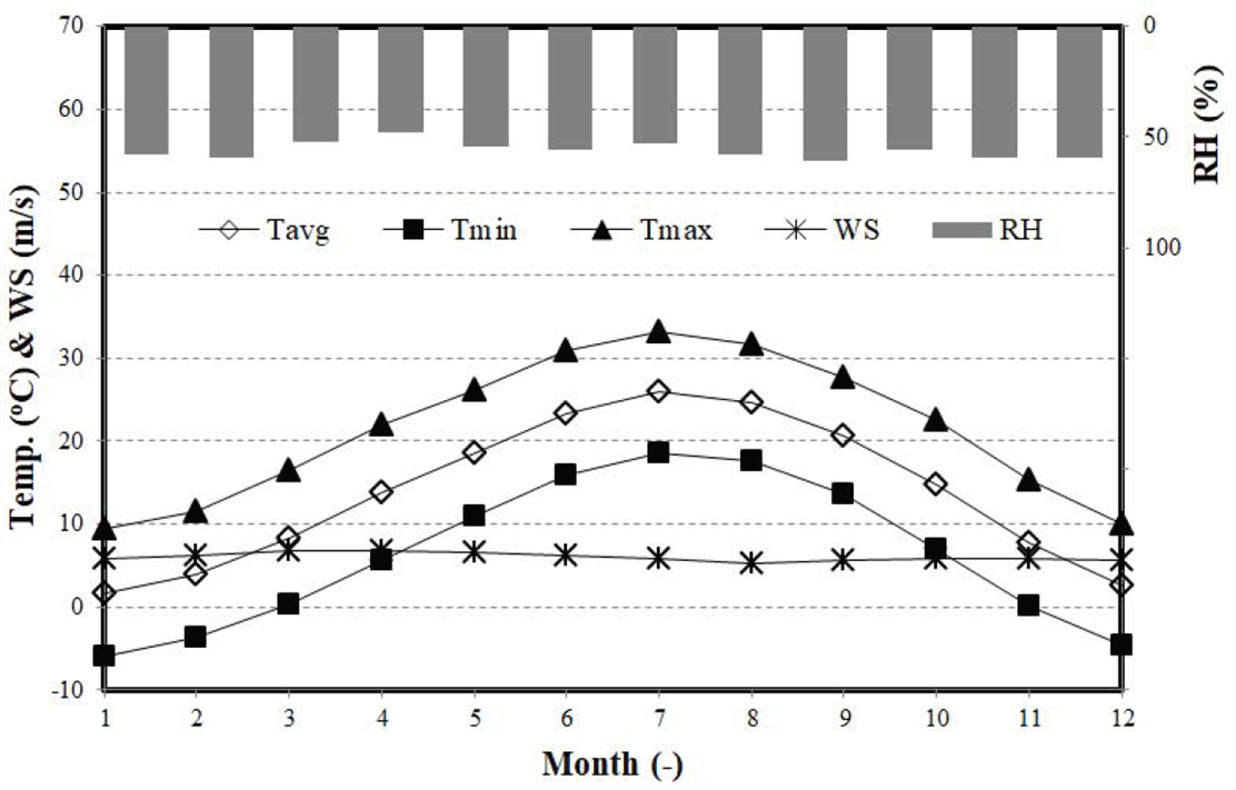
Table 2 presents the maximum, minimum, average and standard deviation (S.D.) values of temperature, relative humidity, wind speed, solar radiation and ETo for the period of study. The multi-year average data for each meteorological variable were 17.13 oC (-14.57~30.85 oC) for Temp., 51.30% (7.40~99.92%) for RH, 5.16 m/s (0.31~9.67 m/s) for WS, 12.22 MJ/m2/day (0.81~27.38 MJ/m2/day) for SR and 4.66 mm/day (0.20~8.97 mm/day) for ETo, respectively.
Table 2
Statistical parameters of daily meteorological variables in study area
2. Relationship between meteorological variables and ET o
Correlations of meteorological variables with ETo are presented in Table 3. This table shows that the linear correlation between meteorological variables with ETo ranged from 0.161 to 0.793. SR has the highest correlation with ETo, which was followed by Tmax, Tavg, Tmin, RH and WS. This indicates that any BPNN and MLR models that use SR and Tmax and/or Tavg as inputs may be able to estimate the ETo to acceptable accuracy, depending on the specific application. The model’s accuracy can be improved by implementing other variables that have aerodynamic effects of ETo, such as RH and WS.
3. Performance comparison between BPNN and MLR models
There is no established methodology for the selection of the appropriate network architecture before training (Coulibaly et al., 2001; Jain et al., 2008; Wu et al., 2014). Therefore, this study began with evaluating the number of hidden layer and PEs in the hidden layer which exhibit non-linear behavior between inputs and output. All other computational parameters (momentum, learning coefficient ratio, learning rule and transfer function) were also determined. The best performance per each combination was achieved and listed in Table 4. The trial and error procedure per each combination (C1 through C20) showed that just one hidden layer worked best and the number of PEs in the hidden layer ranged from 3 to 9. The best choice of momentum and learning rate are problem dependent and need some trial-and-error before good choices are found. In this study, the momentum that was used to modify the current direction of computational movement in weight space based on previous changes was consistent as 0.4 for all combinations. Most combinations except for C12 showed that the learning rate of 0.5 produced the best results, which indicates that no single value of learning rate was optimal for all combinations. The number of iterations was also considered one of the influencing factors on model performance and the preliminary test showed that more than 50,000 iterations did not improve the model accuracy (data not known). Instead of listing all twenty combinations, only the best performing combination per each group (same number of input variables used) is shown in Table 4, for example, C3 was the best performing combination among C1 through C6.
Table 4
Best architecture of BPNN and its computational parameters
Our analyses with ETo revealed that the performance criteria for the best BPNN model had the architecture of 6-1-1, which had one input layer of 6 neurons, one hidden layer of 1 neuron and one output layer of 1 neuron. The momentum and learning rate were initially set to 0.1 and 0.1, respectively. However, they were manipulated at 10 levels (increasing/decreasing by 0.1 from 0.0 to 1.0) in an effort to find the best configuration (0.4 of momentum and 0.3, 0.5 of learning rate). The optimal momentum and learning rate were finally determined to be 0.4 and 0.3(0.5) depending upon input combinations. In addition, the learning rules were varied, but the transfer function of hyperbolic tangent (Tanh) was superior to other functions.
The ability of BPNN modeling to predict daily ETo values using different combination of input variables was examined and their results are shown in Fig. 4. This figure only shows the case with the best modeling result per each BPNN modeling with different combination of input variables. Differently from the correlative regression results, the maximum air temperature had the greatest influence on ETo estimation when only one input variable was used for simulation. However, in the combinations with more than two input variables, SR showed the largest influence on model accuracy. The BPNN model underestimated and overestimated ETo at higher and smaller values, respectively, which may have resulted from diminished sensitivity of training to the more extreme ETo values. Even under this limitation, R2 values ranged from 0.79 to 0.98.
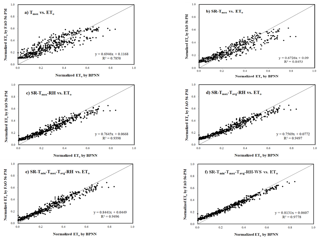
Fig. 4
Scattering diagrams of ETo estimated by BPNN and FAO 56-PM during the testing periods depending upon the combination of input
In this study, the same training and validation datasets with BPNN modeling were used in generating the MLR equations and computing the coefficient of determination at a significance level of 5% between the FAO 56-PM and MLR equations (Table 5). The smallest discrepancies between ETo calculated by BPNN and ETo calculated by the FAO 56-PM equation were achieved from C3, C9, C12, C16, C19 and C20 with 1, 2, 3, 4, 5 and 6 combination of input variables, respectively.
Table 5
Multiple Linear Regression equations per best combination
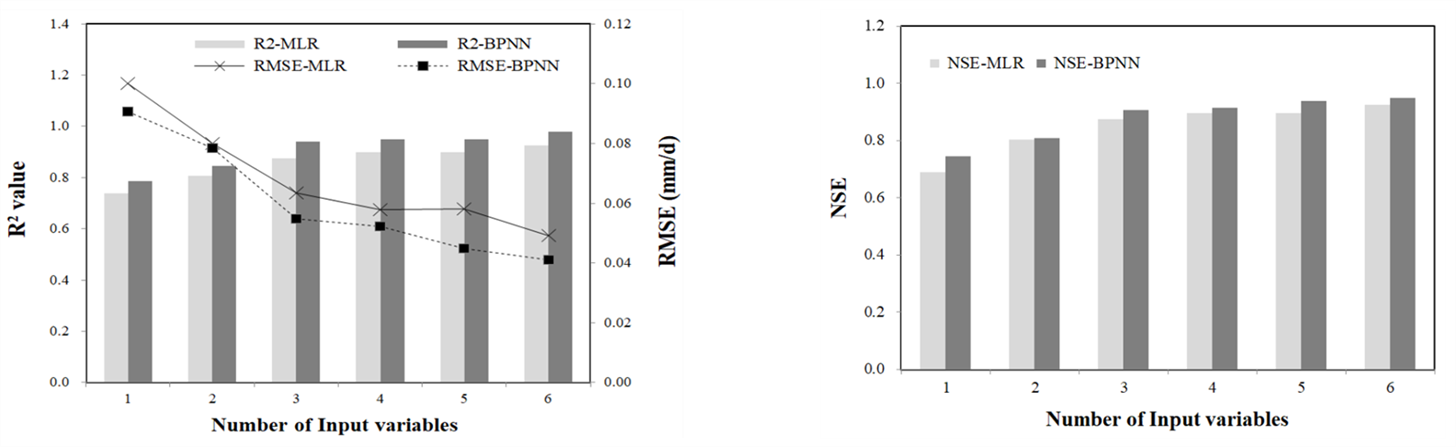
Fig. 5 shows the statistical comparison between BPNN and MLR models depending upon different combination of input variables. The values of R2, RMSE and NSE from BPNN modeling ranged from 0.786 to 0.978, from 0.005 to 0.091 (mm d-1), and from 0.746 to 0.948, respectively. In combination of MLR modeling, values of R2, RMSE and NSE were from 0.738 to 0.925, from 0.049 to 0.100 (mm d-1) and 0.691 to 0.925, respectively. This result showed that BPNN has a better performance than MLR, and both models indicate that no more than three input variables (Tmax, SR, RH) would improve the accuracy.
Ⅳ. CONCLUSIONS
Reference crop evapotranspiration (ETo) plays a major role in the agricultural management of water resources and its accurate prediction would signify better planning and management of the resources. Due to limitations of the FAO 56-PM equation, ANN modeling with BP algorithm was proposed as an alternative in this study to calculate ETo.
A total of twenty combinations with different combination of input variables were carefully selected and tested with ETo as an output. Both BPNN and MLR modeling provided the best results in ETo estimation using all meteorological variables as inputs, which was consistent with a study by Goel (2009) and Benzaghta et al. (2012) indicating that a combination of all input parameters provides better performance of the ANN model in estimating the ETo rather than individual parameters. However, this study found that even three most crucial inputs, Tmax, RH and SR, when used in both BPNN and MLR models to accurately estimate ETo. This result was consistent with a study by Laaboudi et al. (2012). They were able to improve the temperature-based accuracy of a model using incomplete meteorological variables (air temperature, wind velocity and relative humidity) with the proper choice of ANN architecture. Also, they found that the temperature-based accuracy on ETo estimation was improved by incorporating with wind velocity and relative humidity as the network input datasets.
A study by Landeras et al. (2008) compared between ANNs and alternative evapotranspiration equations with lower input requirements to the FAO 56-PM equation. They found that ANNs based on the same inputs, as those required for the application of the FAO 56-PM equations with or without solar radiation or relative humidity, gave a better performance than their analogous linear calibrated equations (the FAO 56-PM based equation with estimated solar radiation and/or relative humidity).
However, it should be noted that the correlation between ETo and meteorological variables could be different over regions, which means that the highest and lowest correlations with ETo were SR and WS in this study, but it could be different in other area. This indicates that it should include more data to train, validate and test BPNN to function as a universal model.
Overall, this study showed that the possibility of estimating ETo with lesser number of meteorological variables as inputs and could provide valuable information on irrigation scheduling in an easily accessible way.