

Ⅰ. INTRODUCTION
Nutrients export from agricultural lands is a significant contributor to the accelerated eutrophication of water bodies globally (Kim et al., 2006). Among the agricultural non-point sources (NPS), paddy fields account for a considerable portion of agricultural land in some East Asian countries (Takeda and Fukushima, 2006). Paddy fields accounted for 54.1% (0.91 million ha) of the agricultural area (1.64 million ha) in South Korea (MAFRA, 2015). The reduction of nutrient loads from paddy rice cultivation, particularly in the Asian monsoon region, has been an essential issue for surface and groundwater water quality management (Zhang et al., 2011). Kim et al. (2007) reported that NPS pollution from paddy fields is a significant problem in water quality management in South Korea. Thus, the government has emphasized to cut nutrient export from paddy fields under the total maximum daily load policy in Korea (Choi et al., 2015).
The downstream water quality may improve by reduction of surface drainage during paddy rice cultivation. It can be achieved by water-saving irrigation, reducing pond water depth, raising the outlet height of paddy fields, and minimizing forced surface drainage (Yoon et al., 2006; Jang et al., 2012; Choi et al., 2013). Matsuno et al. (2006) proposed that appropriate paddy management, including judiciously use of fertilizer, reuse of discharge water, and plot-to-plot irrigation, can considerably reduce water quality problems.
A good number of computer models have been developed to simulate the different aspects of rice cultivation, such as phonological stages, water management, and ecological impacts of rice production. Some models emphasis on predicting rice crop growth and yield, while taking into considering several aspects of water, nutrient, and associated biophysical routes (Tang et al., 2009; Ahmad et al., 2012). Other models are supposed to simulate hydrologic balance, pesticide fate and transport, or the transportation of other pollutants within rice paddies (La et al., 2014; Jeon et al., 2005). As a domestic experiment, CREAMS-PADDY (Seo et al., 2002) has been developed to consider water balance and quality schemes in the paddy field and applied to estimated pollutant loads from the fields (e.g., Song et al., 2011; Kim et al., 2015). These models are used to single rice paddies or clusters of rice paddies within relatively small areas, although few models have been extended to support watershed-scale applications (Tsuchiya et al., 2015; Lee et al., 2018). However, the comprehensive assessment of paddy water quality dynamics based on cropping systems simulation has been limited because some models are capable of simulating the effects of paddy management on biophysical processes in an integrated modeling framework at the field-to-watershed-scale (Tsuchiya et al., 2015).
The Agricultural Policy/Environmental eXtender (APEX) model was developed by integrating single-field functionalities of the Environmental Policy Integrated Climate (EPIC) model and extending them to allow simulations at the field scale, farm scale, and at the small watershed scale. These models have been used to estimate the effects of management changes in a landscape (Havlik et al., 2011), to predict sediment and nutrient loss (Kiniry et al., 1995; Ramirez-Avila et al., 2017), and to estimate the risks of climate change on runoff and nutrient flows (Rosenzweig et al., 2014). However, the APEX model could not simulate paddy-specific practices such as puddling, flood irrigation management, or transplanting, making it difficult to apply the model to rice paddy dominant agricultural watersheds that a recommend to Korea. The Rural Development Administration (RDA), along with Texas A & M University jointly revised the model to allow for the evaluation and management of nonpoint sources in response to the paddy growing environment. Recently, Choi et al., 2017 constructed a physically-based modeling framework for simulating paddy processes by the link in agricultural management practices, including puddling, flood irrigation, transplanting, fertilizer application on flooded paddies, and irrigation management to rice growth and water quality dynamics within the APEX model. They also developed crop parameters that represent the growth characteristics of paddy rice. Up to date, Choi et al. (2017) have been only calibrated the model using the monitoring data from Korean paddy field. They evaluated the APEX-Paddy model and found the APEX-Paddy showed higher accuracy in flow and water-soluble nitrogen prediction. Therefore, further study should be needed within APEX that enhances water quality simulation in rice paddy farms based on algorithms that connect paddy practices, rice growth, and water quality processes at the field-to-watershed scale.
The objectives of this study to evaluate the paddy module using field data from experimental paddy fields in Korea. Experimental fields in the Iksan regions in Korea were selected to test the performance of the paddy module.
Ⅱ. MATERIALS
1. Paddy field experiment data
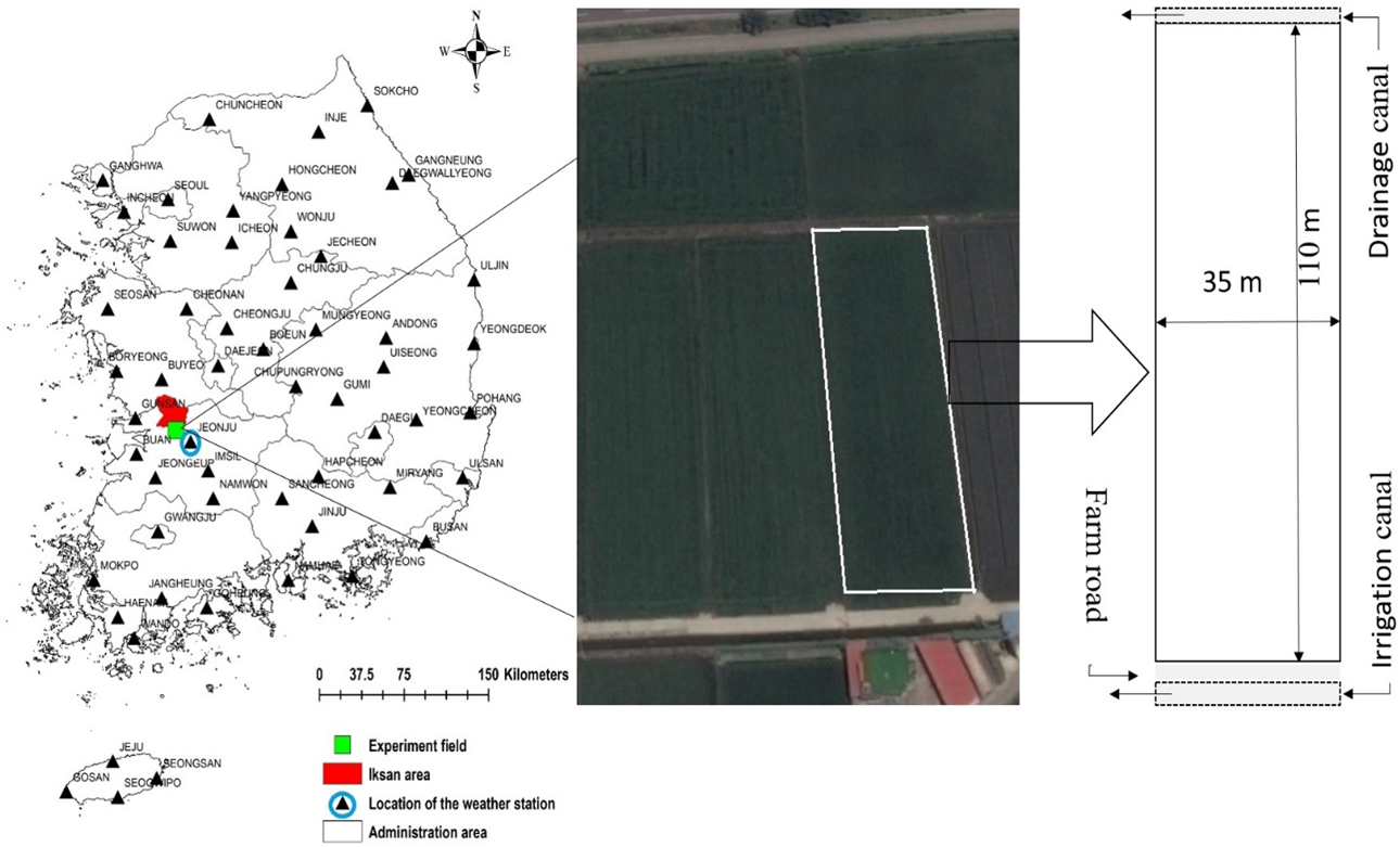
Seoul National University conducted this experiment during the paddy growing season in 2013, and 2014. The experimental field was located near Iksan city (35.9016 N, 127.0331 E) of the Jeonbuk province in South Korea. In terms of soil, Jeonbuk series fits the predominant soil characteristics near the Iksan site. The Jeonbuk series is a poorly drained silty clay loam soil series built on the fluvio-marine plain. The physical properties of the upper layer(~20 cm) of soil contained 11.1 % sand, 71.1% silt, and 17.8% clay. The average annual rainfall is 1260 mm, and the average annual temperature is 12.7°C (https://en. climate-data.org/asia/south-korea/jeollabuk-do/iksan-si-4130/). The study site is highly influenced by the monsoon rainfall. Most of the precipitation occurred in Korea during July and August. Approximately 52% of the annual rainfall occurs in the study area during this time. Most of the growing season for rice includes the monsoon period. Therefore, paddy fields are vulnerable to discharging sediment and nutrients to downstream water bodies.
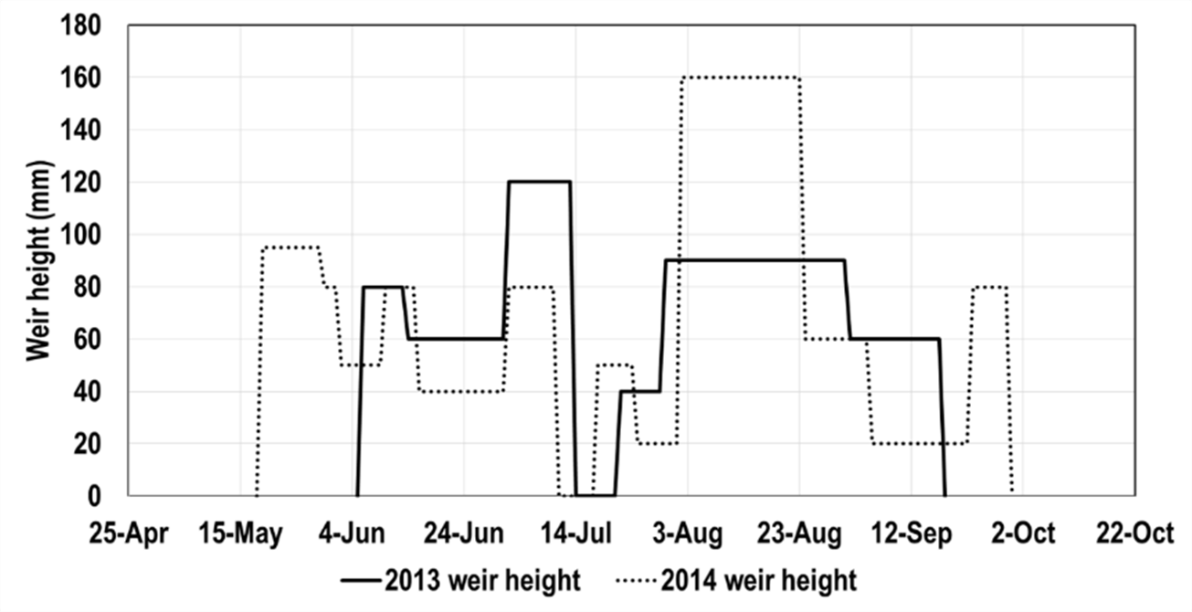
A paddy field of 35 m wide and 110 m long in size was established for paddy hydrology and water quality monitoring, as shown in Figure 1. A weir was also installed at the paddy field drainage outlet to measure the drainage water amount. The outlet weir is also used to control the ponding depth inside the paddy field. Figure 2 illustrates the weir setup in different two years. An ultrasonic water level gauge was used to measure paddy ponding depth. The water samples of paddy fields were collected at regular intervals of 15 days. However, rainfall-runoff samples were collected when the major storm occurred. All water samples were analyzed using standard methods, as described in APHA (1998) for nutrient content determination. The field experiment was performed for two years (2013-2014) during the rice-growing season. Table 1 summarizes the paddy management scheduled during the study period. A Japonica rice variety of ‘Saenuri’ was transplanted as per schedule. Midseason forced surface drainage of 1 to 2 weeks is a common practice in Korea for improving air supply to the rice root zone and increasing the number of tillers for lodging tolerance with sturdy rice stalk (Hong et al. 2012). The forced drainage was practiced in the second week of July for about two weeks.
Table 1
Typical paddy management schedule of the Iksan field
2. APEX-Paddy model setup and inputs
Apex model (version 1501) was used in this study. The APEX-Paddy (modified APEX) model requires inputs site-specific inputs data for simulating discharge, sediment, and nutrients loss from paddy management practices. Soil characteristics are essential factors when modeling runoff from a basin. The U.S. Natural Resource Conservation Service (NRCS) classifies soils into four hydrologic groups based on the infiltration characteristics of the soils. NRCS Soil Survey Staff (1996) defines a hydrologic group as a group of soils having similar runoff potential under the same storm and cover conditions. Soil properties that influence runoff potential are those that impact the minimum rate of infiltration for a bare soil after prolonged wetting and when not frozen. These properties are depth to the seasonally high water table, saturated hydraulic conductivity, and depth to a very slowly permeable layer. Hydrologic soil groups are classified as either an “A”, “B”, “C”, or “D” soil. For instance, “A” soils infiltrate rainwater the best, and therefore properties with an “A” soil generate the least amount of runoff.”D “soils have the lowest infiltration rates and thus contribute the most runoff. In this study, the hydrologic soil group selected ‘B’ due to a terrace that had been installed.
In APEX, a user may either create a new weather station or use one of the default stations defined by the program (Steglich et al., 2016). As APEX works on a daily time-step, a daily weather file (.DLY) was created by using Jeonju weather station data from 1976 to 2015 in this study. Six parameters are used in the weather file, including precipitation, maximum and minimum temperature, solar radiation, relative humidity, and wind speed.
The schematic of the APEX processes with the paddy module is illustrated in Figure 3. With the paddy enhancement, a subarea is flexible for setting land as dry or wet (flooded) as prescribed in the operation schedule file that is attached to the subarea. APEX uses the Natural Resources Conservation Service Curve Number (CN) equation (Hawkins et al. 2009) or the Green and Ampt method for estimating the runoff. The CN technique was selected in this study. The CN method relates run-off to soil type, land use, and management practices (Williams et al. 2008). The APEX model has five options for estimating potential evapotranspiration (PET), such as Penman-Monteith, Penman, Priestley-Taylor, Hargreaves, and Baier-Robertson. In this study, Hargreaves and Samani (Hargreaves and Samani 1985) equation was used for the estimation of PET. Hargreaves is a temperature-based model and uses temperature and extraterrestrial radiation to estimate daily PET. The Hargreaves method gives the best estimate of PET when data on relative humidity, solar radiation, and wind speed data are not available (Williams and Izaurralde 2005).
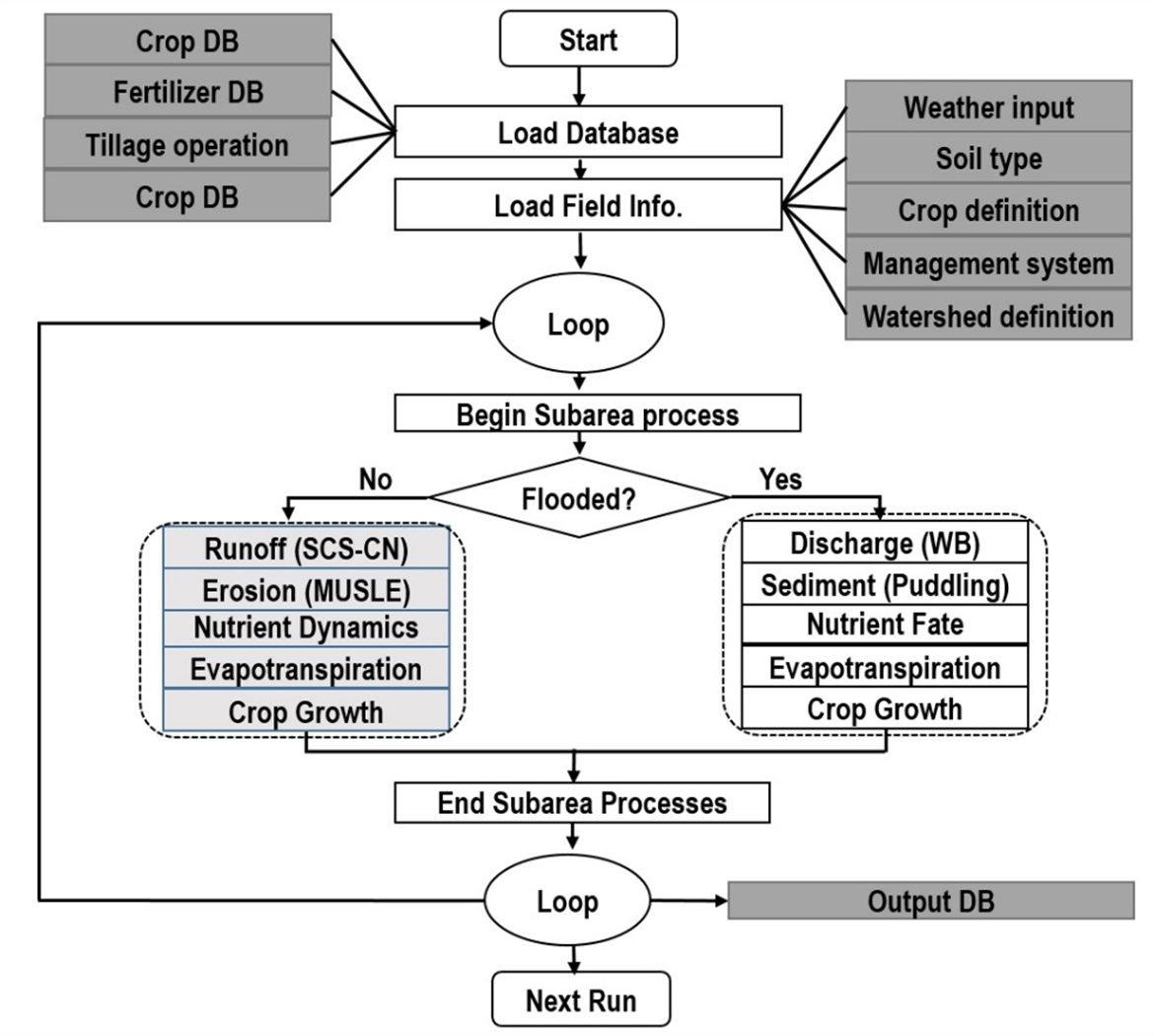
Fig. 3
Schematic diagram of the Agricultural Policy/Environmental eXtender (APEX) ‐Paddy algorithm (Modified from Choi et al. 2017)
There are seven equations to select from in APEX to simulate rainfall/runoff erosion. All of the options are modifications of the Universal Soil Loss Equation (USLE), primarily in the energy component (Steglich et al., 2016). For this research, soil erosion is estimated by the Modified Universal Soil Loss Equation (MUSLE) equation.
The amount of NO3-N lost when water flows through a layer is estimated by considering the change in concentration. Thus, the equation:
Where; QNO3 is the amount of NO3-N lost from a soil layer, and CNO3 is the average concentration of NO3-N in the layer during the percolation of volume QT through the layer.
A loading function developed by McElroy et al., (1976) and modified by Williams and Hann (1978) for application to individual runoff events is used to estimate organic N loss. The loading function is
Where YON is the organic N runoff loss in kg ha-1, Y is the sediment yield in t ha-1, CON is the concentration of organic N in the topsoil layer in g t-1, and ER is the enrichment ratio. The enrichment ratio is the concentration of organic N in the sediment divided by that in the soil.
Calculating P loss in APEX is dependent upon the partitioning of P between the soluble and sediment-bound phase when soil erosion occurs. It’s expected that the majority of P loss occurs in the sediment-bound state (Hansen et al., 2002). Therefore, total P (T-P) loss is significantly affected by the water erosion equations and the concentration of sediment in runoff. Sediment-transported P is simulated with loading functions in APEX and is influenced by the concentration of P in topsoil (Williams et al., 2012). The loading function is estimated by dividing the concentration of organic P in sediment by the concentration of P in the mineral soil. Soluble P loss in surface runoff is calculated using the GLEAMS (Groundwater Loading Effects of Agricultural Management Systems) equation. The GLEAMS equation estimates soluble P loss based on runoff volume, the concentration of labile P, and a ‘Kd’ value. The Kd value is the P concentration in the sediment divided by that in the water (Williams et al., 2012).
Ⅲ. METHODOLOGY
1. Warm-up period selection
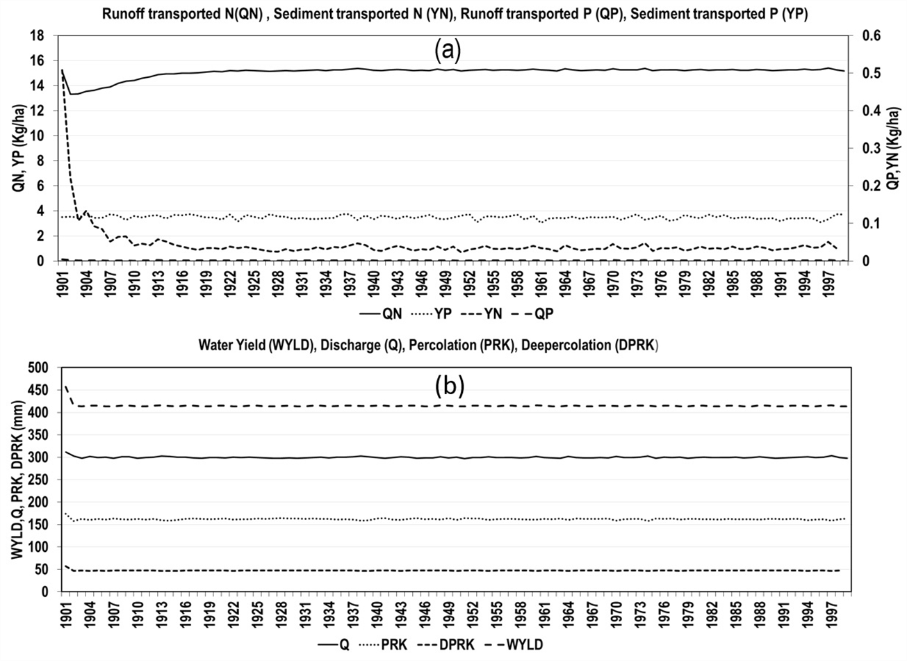
The warm-up time is the time that the simulation will run before starting to collect results. A warm-up period can be essential for successful model performance. Insufficient warm-up periods may result in the early years of the simulation, having biased responses. Therefore, 1 to 4 years of warm-up simulations are common for watershed-scale modeling (Douglas-Mankin et al., 2010). For this research, the model was run for 99 years using the same management and weather data. It was found that after 30 years, the water and nutrients related variables were reached in stable condition. The field operation schedules for two years, and fifteen rotations were simulated. Therefore, model outputs contained data for 30 years, but only the last rotation was assessed (e.g., a simulation lasting from 1984 to 2014, data were evaluated from 2013 to 2014).
2. Sensitivity analysis
As calibrating a model with more number of parameters is a difficult task, a sensitivity analysis was done to reduce the calibration effort. The parameter selection for sensitivity analysis was made based on the characteristics of the study area as well as the literature review. In this study, a sensitivity analysis was conducted using the APEX-CUTE tool. APEX-CUTE offers a sensitivity analysis using the Morris method (Morris, 1991). Then, an investigation was conducted to determine the rate of change in model outputs based on the degree of change to the value of a sensitive parameter. This step is essential to identifying and defining parameters that influenced the model outputs most (Duggupati et al., 2015).
3. Calibration of Parameters
The adjustment of variables that describe site conditions and characteristics is key to fine-tuning calibration. These parameter values are edited in several files, including the subarea file (.SUB), parameter file (.PARM), and control file (CONT). The PARM file is a critical part of the APEX model, containing 110 equation coefficients, exponents, and ratios. These values were manipulated with extreme caution. Sensitive parameters value were determined through trial and error method in manual calibration. The calibration process involved editing parameter values, running the model, and assessing the results. Continued changes in parameter values depended on the over or under-prediction of the model results. Successful calibration occurred when both of the managements met the performance measures as described in ‘Model Evaluation’. It’s important to note that the calibration of the water balance was conducted first and foremost, because sediment, N, and P calibration are dependent on runoff loss.
After calibrating using the trial and error method, an automatic calibration was performed to improve model predictions. The auto-calibration was completed using APEX-CUTE 4.1 (APEX-auto-Calibration). This software uses a Dynamically Dimensioned Search (DDS) algorithm, which repeatedly interacts with the input files, edits parameter values slightly, and runs the model (Wang and Jeong, 2016). The user specifies the number of iterations conducted by the DDS, but it is recommended that this value be set between 500 and 5000 (Wang and Jeong, 2016). The parameters that were allowed to be changed by the auto-calibration software were identified during the manual calibration. The starting values for all parameters were the values used in the manually calibrated model. In this study, 900 iterations were run, and one set of parameters was selected based on the calculated objective function value and best objective function value. Inputs in the soil and management files were not considered for calibration, as those were determined based on measured data or field descriptions during the model setup.
A successful calibration of the APEX Model required the adjustment of model parameters concerning the evaluation criteria for simulating runoff, sediment, T-N, and T-P. The calibrated model used nearly identical parameter values, despite variations in management operations and fertilizer application rates.
4. Model Evaluation
Analyzing model performance after calibration is necessary to quantify relationships between simulated and collected data. It is recommended that both graphical techniques and quantitative statistics be used in model evaluation (Moriasi, 2007). Three different evaluation statistics were used to quantify this study, including coefficient of determination (R2), Nash-Sutcliffe Efficiency (NSE), and Percent Bias (PBIAS). One of the most commonly used criteria in model performance is the R2 correlation coefficient, which is used to determine the goodness of fit (e.g., Moriasi et al., 2015). Values for R2 (bound by 0 and 1) that are closer to 1 indicate a better fit, with an amount of 1indicating a perfect match for comparing predicted values to observed data.
The efficiency of model performance is typically measured after calibrating a model or when processing data (Moriasi et al., 2007). The NSE equation is used to estimate efficiency, and also determines how well the simulated values mimic observed data. These values range from 1 to -∞. Similar to R2 values, an NSE value of 1 indicates a perfect fit, and if NSE is 0, then the simulation is no more accurate than the mean of the data that was observed (Mudgal et al., 2010).
The last statistical measure, PBIAS, describes the tendency of simulated data to over or under-estimate compared to the corresponding observed data (Moriasi et al., 2007). Ideal values of PBIAS are at or near zero, with lower values indicating more accurate simulations. Negative values indicate that the model underestimated the measured data, and positive values correspond with model overestimation bias.
In the equation, x and y are the predicted and observed values,  and
and  are the means of x’s and y’s
What constitutes a successful calibration depends on several factors, including what independent variables are being observed (e.g., runoff volume, nutrient concentration or load, and the period that’s being evaluated). Continuous model development and improvement have influenced acceptable values. In this study, Moriasi et al. 2007 recommended statistics are used, as shown in Table 2.
Table 2
Recommended statistics for the watershed model (Moriasi et al. 2007)
Ⅳ. RESULTS AND DISCUSSIONS
1. Sensitivity analysis
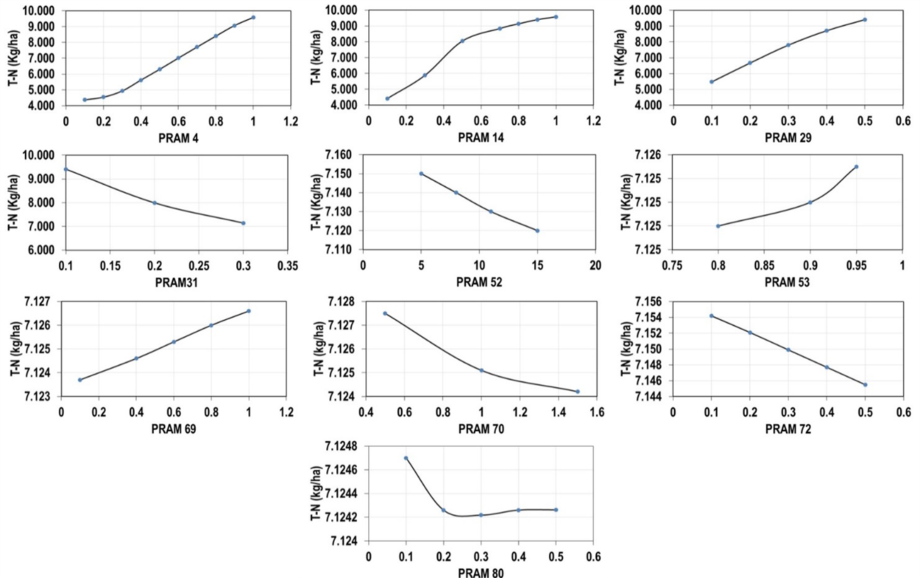
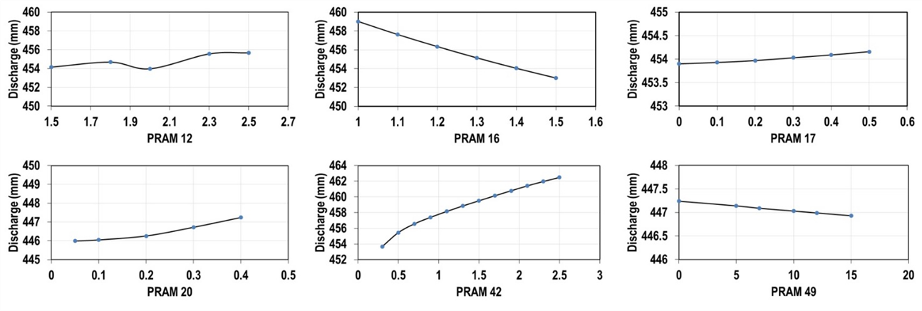
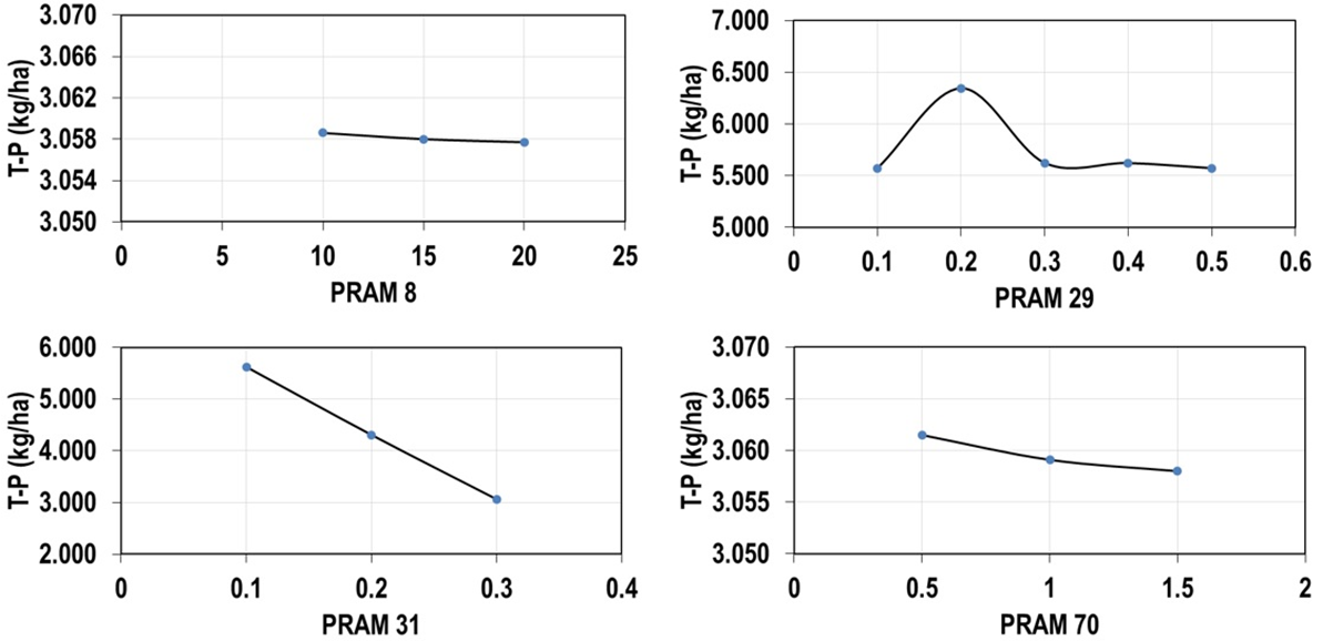
The effects of the parameters were assessed for APEX-Paddy model outputs of discharge (Q), total N loss in runoff (T-N), and total P loss in flow (T-P). Overall, 18 sensitive parameters were detected using APEX-CUTE auto-calibration tools; among them, nine parameters are sensitive to discharge, ten parameters are sensitive to nitrogen yield, and three parameters are sensitive to phosphorus yield. However, PARM 29 and PRAM 31 both are susceptible to nitrogen and phosphorus yield (Table 3). In this study, MUSLE equation used for measuring sediment loss. However, sediment loss influential parameters were not found in the sensitivity analysis. These APEX outputs are of considerable interest to the national assessment.
Table 3
Sensitive parameters considered for calibration of the model
Parameter importance (or sensitivity) can then be assessed by visual inspection of the scatter plots for objective function values or the model output variables versus each parameter value, as shown in Figure (4-6). However, during DDS optimization, it should be noted that a particular parameter value most likely changes simultaneously with other values. Therefore, the changes in different parameter values and significant interactions among parameters also contribute to the changes in model output.
2. Manual Calibration
Based on the results of sensitivity analysis, The APEX- PADDY model was calibrated based on daily discharge (Q), nitrogen yield (T-N), sediment yield (SS), and phosphorus (T-P) yield rates data that were measured at the outlet of the paddy field during the cropping period of 2013 and 2014. Table 4 shows a statistical summary of the calibrated model performance, and Figure 8(a-d) shows comparisons of the observed and simulated discharge, nitrogen yield, sediment, and phosphorus yield, respectively. The manually calibrated model satisfactorily simulated the discharge and nitrogen yield. However, the simulation results of sediment and phosphorus yield were not satisfactory level.
Table 4
Performance statistics for the manually calibrated APEX-Paddy model, including the coefficient of determination (R2), Nash Sutcliffe model efficiency equation (NSE), and Percent Bias (PBIAS) (Individual year and entire calibration period)
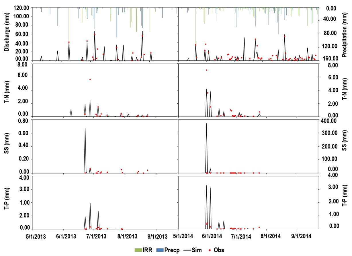
Fig. 8
Observed and simulated daily (a) discharge, (b) nitrogen yield, (c) sediment yield, and (d) phosphorus over the manual calibration period of the paddy the growing season in 2013, and 2014
As depicted in Table 4, the performance of the paddy model is demonstrated to be satisfactory in predicting runoff discharge rate (R2 = 0.78, NSE = 0.65, PBIAS = 5.41%), which proves that the simulation effectively reflects the field data. These results show that the APEX-Paddy model successfully calibrated discharge. For T-N, the performance statistics demonstrated to be satisfactorily predicting the nitrogen yield (T-N) rate (R2 = 0.51, NSE = 0.68, PBIAS = 20.93%), proves that APEX-Paddy model successfully calibrated the nitrogen yield. According to performance statistics, simulation data of sediment and phosphorus had shown the overestimated values, which demonstrates that the simulation is not effectively reflects the field data. Results indicate that the APEX-Paddy model did not successfully calibrate the sediment and phosphorus yield. It might be happened due to the limitation of the sediment routine of the model. It will discuss in detail later part of the article.
3. Auto-calibration
The model parameters modified using an auto-calibration tool (APEX-CUTE 4.1) for predictions of runoff, sediment, N, and P. Of the 900 iterations of APEX runs, the set of parameters that resulted in the best model occurred within the first 225 runs. The parameters from the best run were applied and used to calculate model performance. Table 5 shows a statistical summary of the model performance, and Figure 9(a-d) illustrates the comparisons of the simulation and observation, as shown in Figure 8 but for the results of auto-calibration. Similarly to the results for manual calibration, while the automatic calibration systems also performed reasonably in the calibration of runoff and nitrogen yield, the performance statistics indicated the unsatisfactory simulation of sediment and phosphorus yield.
Table 5
Performance statistics for the Auto-calibrated APEX-Paddy model, including the coefficient of determination (R2), Nash Sutcliffe model efficiency equation (NSE), and Percent Bias (PBIAS) (Individual year and entire calibration period)
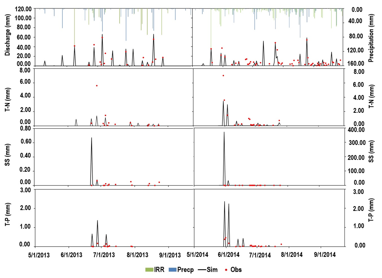
Fig. 9
Observed and simulated daily (a) discharge, (b) nitrogen yield, (c) sediment yield, and (d) phosphorus over the automatic calibration period of the paddy the growing season in 2013, and 2014
As shown in Table 5, the performance of the paddy model is demonstrated to be satisfactory in predicting runoff discharge rate (R2 = 0.78, NSE = 0.65, PBIAS = -6.39%), which proves that the simulation effectively reflects the field data. These results confirm that the APEX-Paddy model successfully calibrated discharge. For T-N, the performance statistics demonstrated to be acceptably predicting the nitrogen yield (T-N) rate (R2 = 0.51, NSE = 0.64, PBIAS = 44.09 %), shows that APEX-Paddy model successfully calibrated the nitrogen yield (T-N). The simulated value of sediment and phosphorus yield are not meet the statistically satisfactory level both individual management practice in two different years and the entire period as well, except the R2 value of T-P in 2013. Simulation results of sediment and phosphorus had shown the overestimated values, which shows that the simulation is not effectively reflects the field data. It indicates that the APEX- Paddy model did not successfully calibrate the sediment and phosphorus yield. It might be happened due to the limitation of the sediment simulation component of the APEX-Paddy model. It is discussed in detail the “limitation” part of the article.
The manually calibrated model performed better than the automatically calibrated model in nearly all comparisons. For runoff, R2, and NSE values of automatically calibrated model were the same as the manual calibration. However, a little improvement has shown PBIAS in manual calibration in the entire period. For T-N, NSE and PBIAS values have demonstrated improved results in manual calibration in the whole period, whereas R2 value was the same as manual calibration. Previously, a study was conducted by the University of Wisconsin-Green Bay, USA (Kalk, 2018) for evaluating the APEX model to simulate runoff, sediment, and phosphorus loss from agricultural fields and showed that the performance of a manually calibrated model better than the automatically calibrated model.
4. Limitation of Model
The main limitation of the APEX-Paddy model is the prediction of sediment yield. The APEX component for water-induced erosion simulates erosion caused by rainfall and runoff and by irrigation (sprinkler and furrow). To simulate rainfall/runoff erosion, APEX contains seven equations- Universal Soil Loss Equation (USLE); Onstad-Foster (AOF) version of USLE; Modified USLE (MUSLE & RUSLE); and three MUSLE variants, MUST, MUSS, and MUSI (Wischmeier and Smith, 1978; Onstad and Foster, 1975; Renard et al., 1997; Williams, 1975)
In this study, MUSLE equation is used to simulate erosion and sediment yield. MUSLE estimates the sediment yield by calculating the tons of soil lost through sheet and rill erosion processes on a daily basis. This equation includes sheet and rill erosion that occurs when precipitation is sufficient to result in surface water runoff. The sheet and rill erosion may occur in upland condition only. However, paddy rice management practice is quite different from upland crop management. Traditionally the paddy fields are earth-bermed by 10-30 cm in height and are flooded to 3-10 cm deep for the most of the growing season in Korea. MUSLE or other erosion models do not works when a paddy field is inundated (ponded condition) because these models are developed for estimating soil erosion by surface runoff.
A tillage operation, while a paddy is inundated, will make the paddy water well mixed with topsoil to form dense, muddy water. The model reproduces what would happen when soils are tilled while having ponding water in the field, or puddled. These conventional erosion methods become active after a “destroy puddle” command in the OPS file (The operation schedule file). Sediment concentration of paddy water is influenced by puddling operation. After puddling, the sediment concentration of the paddy water becomes very high and then exponentially reduces over the next multiple days. Thus, if there happened storm events right after a puddling operation that creates overflow, a significant amount of sediment discharged from the paddy field. Conversely, if the storm events happened after some days of puddling operation and created overflow, a very minimum amount of sediment discharged from the paddy field, as shown in Figure 10.
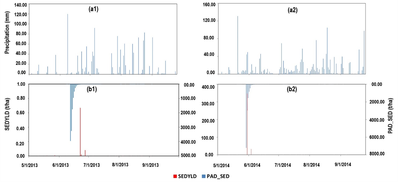
The runoff occurring time is the main factor of sediment yield during the growing season, which is controlled by the weir height setup. When applying for long term simulation such as climate change forecasts, the modeling with the fixed weir height control setup may not simulate relevant sediment yield for the entire simulation period due to the different rainfall patterns at annual basis.
It is well known that up to 90% of the phosphorus transported from cropland is attached to sediment (Sharply and Beegle, 2001). Soil erosion rate directly influences the phosphorous yield calibration. Therefore, it is essential to calibrate phosphorus yield after get the soil erosion rate well-calibrated.
Ⅴ. CONCLUSION
The APEX-Paddy is the model developed to simulate water balance and quality behavior in the paddy. In this study, the performance of the APEX-Paddy model was evaluated to simulate discharge, sediment, nitrogen, and phosphorus yield using monitoring data at Iksan experimental paddy sites in Korea. Two years (2013-2014) paddy field experimental data were used to both manually and automatically calibrate the model.
The manual calibrated model was able to simulate runoff and nitrogen yield loss from the paddy management field in the study area, as indicated by the selected goodness of fit criteria. For runoff, the R2, NSE, and PBIAS values are 0.78, 0.65, and 5.41%, respectively. For T-N, R2, NSE, and PBIAS values are 0.51, 0.68, and 20.93%, respectively. These results prove that the simulation effectively reflects the field data. The performance statistics of the automatically calibrated model were the same as the manual calibration for simulating runoff except for PBIAS (-6.39%). For T-N, comparatively worsen value of NSE (0.64), and PBIAS (44.09%) have found in automatically calibration system. However, R2 value was the same in both the calibration system. It seems that the manually calibrated model performed better than the automatically calibrated model in nearly all comparisons. However, the performance statistics demonstrated that the sediment yield is not properly predicted due to the limitation of sediment/ water erosion sub-routine in both of the calibration system. As the sediment yield directly influences phosphorus yield, the model is also not reasonably simulated the phosphorus yield.
APEX-Paddy model could be used to predictions of runoff and nitrogen yield in South Korea. Existing models are often less practical for nutrient loading estimates because they are either too sophisticated to simulate various farming conditions and best management practices (Jeon et al. 2005). Therefore, APEX-Paddy could be a useful tool for assessing the BMPs for reducing surface runoff and water-soluble nitrogen from the paddy fields in future climate projections. However, sediment sub-routine may need further improvement in the ability to better-predicting sediment and phosphorus yield as well.